
1. Trend, noise, or reversal?
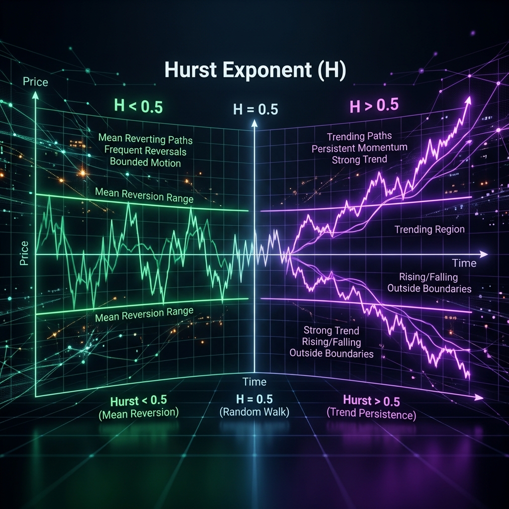
Price series come in three flavours. Some trend: a move up makes the next move up more likely, so trends persist. Some are pure random walk: the next move is independent of the last, and the past tells you nothing. And some mean-revert: a move up makes a move down more likely, so the series oscillates around a level. Which regime you're in decides whether momentum or mean-reversion is the right posture — and getting it wrong is one of the fastest ways to lose money in a live market.
The Hurst exponent, named after the hydrologist Harold Edwin Hurst, collapses that distinction into one scalar between 0 and 1. It measures the long memory of a series: how much the past influences the future, and in which direction.
2. What H actually means
The interpretation is refreshingly direct:
| Hurst H | Regime | Behaviour |
|---|---|---|
| H < 0.5 | Anti-persistent | Mean-reverting — moves tend to reverse |
| H ≈ 0.5 | Random walk | No memory — the efficient-market baseline |
| H > 0.5 | Persistent | Trending — moves tend to continue |
H = 0.5 is the null hypothesis of an efficient market — the same baseline the variance ratio test is built around. Deviations from 0.5 are what a strategy tries to exploit, and the Hurst exponent is one of the cleanest ways to detect and size them.
3. Rescaled range analysis
Hurst's original insight came from studying Nile flood levels, and the method he built — rescaled range (R/S) analysis — is still the standard estimator. The idea is to measure how the "spread" of the series grows as you look at longer and longer windows.
For a window of the series, you first remove its mean, then form the running cumulative sum of those deviations. The range R is the distance between the highest and lowest points of that cumulative path. Divide it by the window's standard deviation S to get the dimensionless rescaled range R/S. Do this over windows of many sizes, and a scaling law emerges:
E[ R/S ]n ∝ nH
The average rescaled range over windows of size n grows like n raised to the Hurst exponent. Take logs of both sides and the relationship becomes a straight line, so H is simply the slope of log(R/S) against log(n), recovered by a linear regression across window sizes.
4. The recipe, step by step
Concretely, estimating H is a short pipeline:
Choose a set of window sizes (typically doubling: 8, 16, 32, …). For each size, split the series into non-overlapping chunks; within each chunk, mean-adjust, build the cumulative deviation path, take its range R and the chunk's standard deviation S, and record R/S. Average R/S across the chunks of that size. Finally, regress the log of those averages on the log of the window sizes — the slope is your Hurst estimate. Because it aggregates behaviour across many horizons, R/S is naturally robust to the sampling choices that plague single-lag statistics; sampling by activity via information-driven bars before you start makes the input cleaner still.
5. Reading H without fooling yourself
The Hurst exponent is powerful but easy to over-read. A few honest caveats:
First, short samples bias H upward. On a few dozen points, even genuine white noise routinely estimates well above 0.5; the classic R/S estimator needs hundreds of observations before it settles, and there are small-sample corrections for exactly this reason. Second, the estimate depends on which window sizes you use and how you handle overlapping data, so it should be treated as an estimate with a confidence band, not a precise constant. Third, apply it to a roughly stationary series — returns, not raw prices; run it on prices and the built-in drift will masquerade as persistence. And finally, H is a description of a regime, not a trading signal on its own: a high H tells you the market has been trending, not that it will keep trending tomorrow.
6. Where it fits in the toolkit
The Hurst exponent belongs to the same family as the market-efficiency diagnostics: it answers the same question as the variance ratio and return autocorrelation, from a different angle, and the three cross-check one another. A strategy developer uses it to pick a regime — deploy momentum where H is persistently above 0.5, mean-reversion where it sits below — and to watch for regime change as H drifts across the 0.5 line over time. It pairs naturally with honest cost measurement too: a mean-reversion edge that H suggests is real can still be erased by the bid-ask spread, so the two analyses belong in the same backtest.
7. Computing it
Estimating H needs only arithmetic — no heavyweight dependencies. Our open-source orderflow-metrics library ships a rescaled-range estimator in both TypeScript and Python:
import { hurstExponent } from "orderflow-metrics";

hurstExponent(returns);
// ~0.5  random walk (efficient)
// > 0.5 persistent / trending
// < 0.5 mean-reverting
// NaN   series too short (needs ~32+ points)
The Python distribution exposes the same function as hurst_exponent. Point it at a rolling window of returns, track how H moves relative to 0.5, and you have a live read on whether the market is trending or reverting — one more lens in the market microstructure stack we build in the open.
8. Conclusion
Trend or mean reversion is the first question every systematic strategy has to answer, and the Hurst exponent answers it with a number instead of a hunch. Above 0.5 the market remembers and persists; below 0.5 it forgets and reverts; at 0.5 it is the efficient random walk that gives no edge at all. Estimate it honestly — on returns, on enough data, with a healthy respect for small-sample bias — and it becomes a compass for choosing the right strategy and spotting when the regime has turned. Explore the rest of the toolkit in our quantitative research library, or read the implementation in our open-source metrics.