
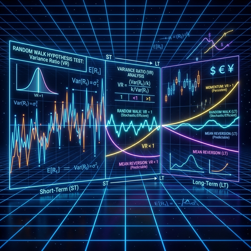
1. Introduction: Deciphering Market Structure
Is a financial market trending, mean-reverting, or simply behaving as a random walk? For quantitative traders, distinguishing between these structural states is critical. If a series behaves as a pure random walk, standard technical signals represent overfitting to white noise. If it exhibits mean reversion or momentum, structured alphas can be successfully extracted.
While many traders estimate autocorrelation coefficients directly, a more mathematically robust answer lies in the **Lo-MacKinlay Variance Ratio Test** (Lo and MacKinlay, 1988). By comparing the scaling properties of variance across different time horizons, this test formally evaluates the Random Walk Hypothesis (RWH).
2. Mathematical Foundations of the Variance Ratio
Let $p_t$ represent the log-price of an asset. Under the Random Walk Hypothesis, log-price increments (returns $r_t = p_t - p_{t-1}$) are independent and identically distributed (i.i.d.). Under this assumption, the variance of $k$-period returns must scale linearly with the aggregation horizon $k$:
$Var(p_t - p_{t-k}) = k \cdot Var(p_t - p_{t-1})$
The **Variance Ratio** $VR(k)$ is defined as the ratio of the scaled variance over $k$ periods to the variance over 1 period:
$VR(k) = \frac{Var(p_t - p_{t-k})}{k \cdot Var(p_t - p_{t-1})}$
The value of $VR(k)$ reveals three distinct structural regimes:
| VR(k) Value | Market Regime | Autocorrelation Signature | Trading Strategy Implications |
|---|---|---|---|
| $VR(k) = 1$ | Random Walk (Noise) | Zero autocorrelation. | Market is efficient; avoid trend-following or mean-reversion trades. |
| $VR(k) < 1$ | Mean Reverting | Negative autocorrelation (anti-persistence). | Favorable for market-making and pairs-trading models. |
| $VR(k) > 1$ | Trending (Momentum) | Positive autocorrelation (persistence). | Favorable for trend-following algorithms and breakouts. |
3. Homoscedasticity vs. Heteroscedasticity
Lo and MacKinlay developed test statistics to verify whether deviations from $VR(k) = 1$ are statistically significant. The test is constructed under two assumptions:
- Homoscedasticity ($M_1$): Assumes return variance is constant over time. The test statistic $z(k)$ follows a standard normal distribution asymptotically.
- Heteroscedasticity ($M_2$): Relaxes the constant variance assumption, adjusting for time-varying volatility clustering (common in financial series). The adjusted statistic $z^*(k)$ is robust to ARCH/GARCH effects.
4. Python Implementation: Lo-MacKinlay Variance Ratio Test
Below is a zero-dependency Python implementation to calculate the variance ratio and its corresponding test statistics:
import numpy as np

def variance_ratio_test(prices, k):
    """
    Computes Lo-MacKinlay Variance Ratio Test for a given horizon k.
    prices: List or 1D array of asset prices.
    """
    log_prices = np.log(prices)
    n = len(log_prices)

    # 1. Base 1-period returns
    returns_1 = log_prices[1:] - log_prices[:-1]
    mu = np.mean(returns_1)
    var_1 = np.sum((returns_1 - mu)**2) / (n - 2)

    # 2. k-period returns
    returns_k = log_prices[k:] - log_prices[:-k]
    var_k = np.sum((returns_k - k * mu)**2) / ((n - k) * (n - k + 1 - k/n))

    # 3. Variance Ratio
    vr = var_k / (k * var_1)

    # 4. Standard Error under Homoscedasticity
    phi1 = (2 * (2*k - 1) * (k - 1)) / (3 * k * n)
    z_homo = (vr - 1) / np.sqrt(phi1)

    return vr, z_homo

# Example usage:
# prices = [100.0, 101.2, 100.8, 102.1, 101.5, 103.0, 102.4]
# vr, z_stat = variance_ratio_test(prices, k=3)
# print(f"Variance Ratio: {vr:.4f} | Z-Stat: {z_stat:.4f}")
5. Conclusion & Open-Source Update
Analyzing return dynamics via the variance ratio provides a mathematically sound basis for strategy selection, avoiding overfitting on white noise. As announced in our latest Open-Source Update, we have integrated these variance ratio models and return autocorrelation modules into our core metrics toolkit.