
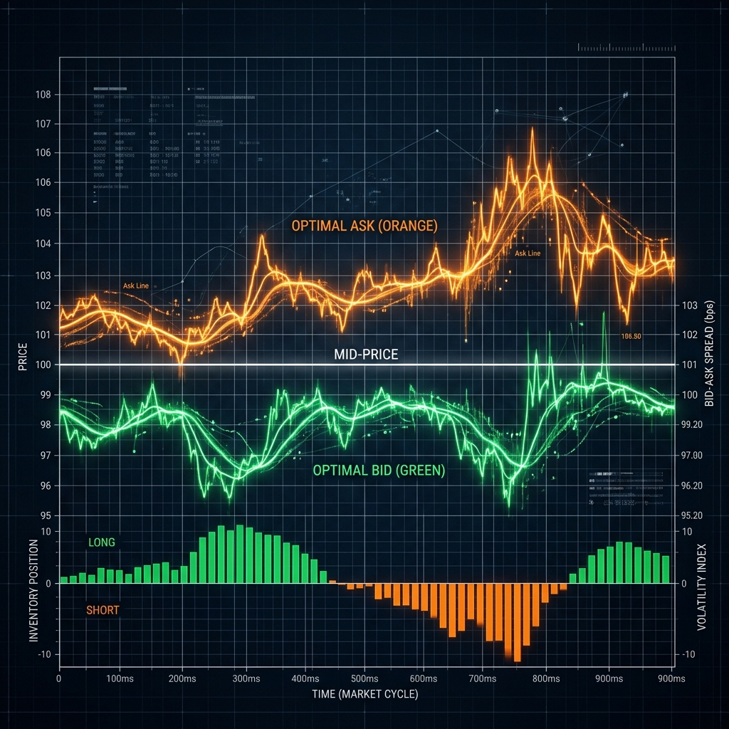
1. Introduction: The Market Maker's Dilemma
A market maker provides liquidity by continuously quoting bids (buy orders) and asks (sell orders) on both sides of the Limit Order Book. The primary source of revenue is the **bid-ask spread**. However, the market maker faces a major structural risk: **inventory risk**.
If the market maker receives consecutive buy orders, they accumulate a short position. If they receive sell orders, they accumulate a long position. If the price moves against this accumulated position before it can be liquidated, the market maker suffers significant losses. Finding the optimal quoting distance to maximize spread revenue while mitigating inventory risk is the central objective of quantitative market-making frameworks.
2. The Avellaneda-Stoikov Model
First proposed by Marco Avellaneda and Sasha Stoikov in 2008, the model calculates optimal quoting spreads based on asset price volatility ($\sigma$), the market maker's risk aversion ($\gamma$), and the remaining time to the trading horizon ($T - t$). Let $s$ be the current mid-price and $q$ be the market maker's current inventory. The model defines the **reservation price** $R$ as:
$R(s, q, t) = s - q \cdot \gamma \cdot \sigma^2 \cdot (T - t)$
The reservation price represents the price at which the market maker is indifferent to adding inventory. If inventory $q$ is positive (long position), the reservation price shifts below the mid-price. This pushes the quoted bid and ask prices lower, discouraging further buys and encouraging sells to revert inventory back to zero.
The optimal spreads $r^a$ (distance to ask quote) and $r^b$ (distance to bid quote) relative to the reservation price are calculated as:
$r^a(q, t) + r^b(q, t) = \gamma \cdot \sigma^2 \cdot (T - t) + \frac{2}{\gamma} \ln\left(1 + \frac{\gamma}{\kappa}\right)$
Where $\kappa$ represents the order book liquidity parameter (the probability of order execution decay as quotes move further from mid-price). The actual quoted bid $p^b$ and ask $p^a$ are:
$p^b = R - r^b \quad \text{and} \quad p^a = R + r^a$
| Inventory State ($q$) | Reservation Price ($R$) | Quoted Ask ($p^a$) | Quoted Bid ($p^b$) | Execution Probability Effect |
|---|---|---|---|---|
| $q = 0$ (Neutral) | Equals Mid-price $s$ | Symmetric distance | Symmetric distance | Equal fill chance on both sides. |
| $q > 0$ (Long) | Shifts below Mid-price | Closer to Mid-price | Further from Mid-price | Higher probability of selling, lower of buying. |
| $q < 0$ (Short) | Shifts above Mid-price | Further from Mid-price | Closer to Mid-price | Higher probability of buying, lower of selling. |
3. Python Implementation: Simulating Reservation Price Shifts
The following Python script computes the Avellaneda-Stoikov reservation price and quoted spreads based on inventory changes:
import numpy as np

def compute_avellaneda_stoikov(s, q, t, t_horizon, volatility, gamma, kappa):
    """
    Computes reservation price and optimal quotes under Avellaneda-Stoikov.
    """
    dt = t_horizon - t
    # 1. Calculate Reservation Price
    r = s - q * gamma * (volatility ** 2) * dt

    # 2. Calculate Bid-Ask Spread width
    spread = (gamma * (volatility ** 2) * dt +
              (2 / gamma) * np.log(1 + gamma / kappa))

    # 3. Calculate Bid and Ask Quote Offsets
    r_half = spread / 2

    p_bid = r - r_half
    p_ask = r + r_half

    return r, p_bid, p_ask

# Example: Mid-price 100.0, Volatility 2%, Risk Aversion 0.1, Liquidity 1.5
for current_inventory in [-5, 0, 5]:
    res_p, bid, ask = compute_avellaneda_stoikov(
        s=100.0, q=current_inventory, t=0.0, t_horizon=1.0,
        volatility=0.02, gamma=0.1, kappa=1.5
    )
    print(f"Inventory q={current_inventory} | Res Price: {res_p:.2f} | Bid: {bid:.2f} | Ask: {ask:.2f}")
4. Conclusion
The Avellaneda-Stoikov framework represents a foundational breakthrough in high-frequency trading mathematics. While real-world market makers incorporate additional parameters (such as adverse selection from order flow imbalance and queue positions), the core concept of reservation price scaling based on inventory constraints remains a critical pillar of risk management.